12.3. Create Denver specific tables

Section 12.2 started a theme of reducing data, with reduced detail for the entire region of Colorado. The goal in Section 12.3 is similar, but different. The goal in this section is to create a data set with detailed data (no aggregation) but limiting it for a smaller, targeted region.

Creating a detailed, targeted data set is often a good idea to do when working on region-scoped projects. It is also helpful, or even necessary, when creating an embedded map solution to reduce the total size of the packaged data. An example of that type of embedded project is found in my blog post qgis2web to export and share interactive maps.

Note

Section 12.3 assumes OpenStreetMap data has been loaded by following the steps outlined in Section 8.

12.3.1. Define goals

Our goal is to provide detailed data for a specific county of interest. The chosen focus for the goal is the City and County of Denver. OpenStreetMap data we want to include:

• Roads

• Natural details

• Water

• Buildings

It is helpful to provide thematic data for some distance outside your main focus. This is helpful when it comes to the stage of creating final outputs. Our thematic data includes our county of focus along with the immediately surrounding counties.

• Counties adjacent to focus

• Thematic major roads

12.3.2. Single County Data

The query in Listing 12.18 creates a schema named osm_denver to save the new data set. It also creates the osm_denver.focus table as an UNLOGGED table that simply defines the area of interest. The focus table is used in the subsequent queries to extract the data of interest.

Listing 12.18 Create osm_denver schema and focus table

CREATE SCHEMA osm_denver;

CREATE UNLOGGED TABLE osm_denver.focus AS
SELECT osm_id, name, admin_level, geom
    FROM osm.vplace_polygon
    WHERE name = 'Denver County'
;

Listing 12.19 creates a primary key and spatial index on the osm_denver.focus table.

Listing 12.19 Create a PRIMARY KEY and spatial index on osm_denver.focus

ALTER TABLE osm_denver.focus
    ADD CONSTRAINT pk_osm_denver_focus
    PRIMARY KEY (osm_id)
;

CREATE INDEX gix_osm_denver_focus
    ON osm_denver.focus USING GIST (geom)
;

12.3.2.1. Detailed roads

Roads are an often-used element in spatial analysis and visualization. Listing 12.9 created a thematic roads table intended for display by filtering for major roads and aggregating them down to their highway names. The goal has adjusted for roads. With this goal, we want to keep all of the detail from the original roads table, only reducing the size of the region the data covers to osm_denver.focus, limiting from all Colorado to only Denver.

Let’s go over three (3) methods for determining which roads are to be included in the reduced table. The three methods examined are:

• Bounding box intersection

• Containment

• Geometry intersection

The first method uses a bounding box intersection query with &&, introduced in Section 7.2.1. Listing 12.20 creates a table osm_denver.road_line_bbox containing all roads where the road’s bounding box overlaps the bounding box for Denver. The image in Figure 12.3 shows the roads included make up a square the size of Denver’s bounding box. Due to the odd shape of Denver’s polygon, the simple bounding box intersection returns a lot of roads to the northwest and southeast that are not associated with Denver itself.

Listing 12.20 Select Denver roads using && bounding box intersection

CREATE TABLE osm_denver.road_line_bbox AS
SELECT DISTINCT r.*
    FROM osm_denver.focus f
    INNER JOIN osm.road_line r
        ON f.geom && r.geom
;

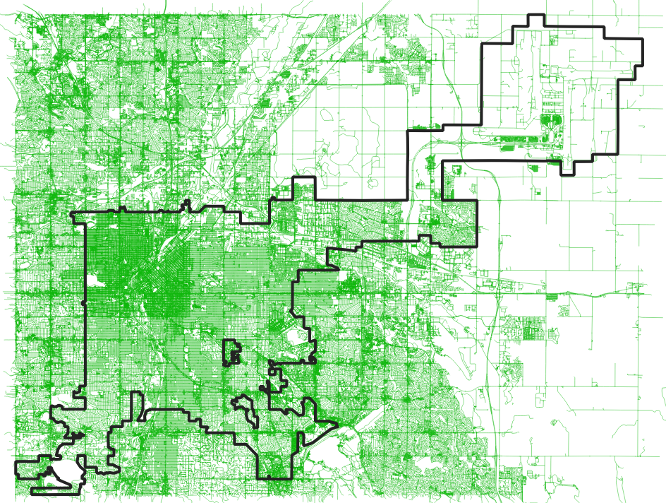
Figure 12.3 Roads returned around Denver County with Bounding Box (&&) query

The simple bounding box intersection used in Listing 12.20 returned too many rows for a Denver-specific data set. Therefore, the second method, shown in Listing 12.21, is updated to use the ST_Contains() function introduced in Section 7.3.1. This change switches from including all roads in the general region to including only roads that are completely within the polygon of Denver. Figure 12.4 illustrates this change in selection with all road lines being fully contained within the polygon for Denver.

Listing 12.21 Select Denver roads using ST_Contains()

CREATE TABLE osm_denver.road_line_contain AS
SELECT DISTINCT r.*
    FROM osm_denver.focus f
    INNER JOIN osm.road_line r
        ON ST_Contains(f.geom, r.geom)
;

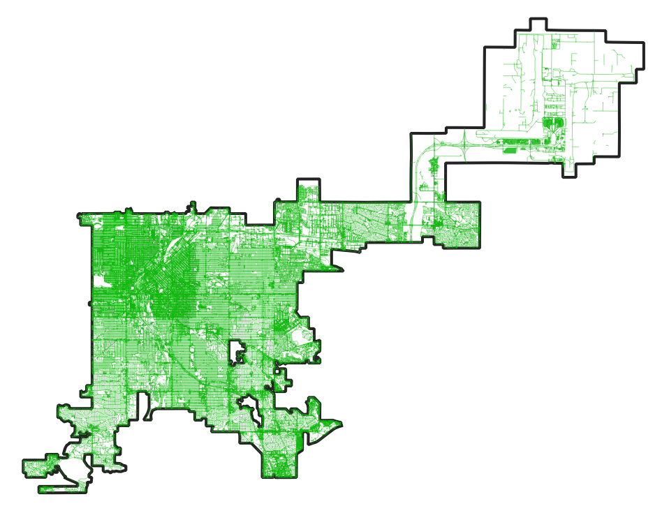
Figure 12.4 Roads returned in Denver County using ST_Contains()

Using ST_Contains() (Listing 12.21) can be too restrictive for some use cases. On the other hand, using && (Listing 12.20) often includes too much data. The third option is a good in-between option to consider: ST_Intersects(). The option using actual geometry intersection is shown in Listing 12.22 with visual results in Figure 12.5. These results show that ST_Intersects() include lines that cross the Denver polygon as well as those completely contained within Denver.

Listing 12.22 Select Denver roads using ST_Intersects()

CREATE TABLE osm_denver.road_line AS
SELECT DISTINCT r.*
    FROM osm_denver.focus f
    INNER JOIN osm.road_line r
        ON ST_Intersects(f.geom, r.geom)
;

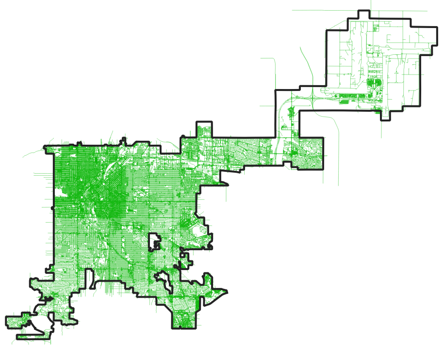
Figure 12.5 Roads returned in Denver County using ST_Intersects()

Note

The table created with ST_Intersects() (Listing 12.22) is simply named osm_denver.road_line and is the version used in later examples.

The query in Listing 12.23 compares the row count and size on disk of the three (3) methods explored. The osm_denver.road_line_bbox table (Listing 12.20) is the more than double the size of the other two tables, with 177,492 rows. The osm_denver.road_line_contain table (Listing 12.21) was the strictest implementation (72,752 rows), excluding any roads that are not fully contained within the Polygon. The difference in size between using ST_Contains() and ST_Intersects() (Listing 12.22) is only about 1,500 rows.

Listing 12.23 Query for row count and size of the 3 road tables

SELECT s_name, t_name, rows, size_pretty
    FROM dd.tables
    WHERE s_name = 'osm_denver'
        AND t_name LIKE 'road%'
    ORDER BY rows
;

┌────────────┬───────────────────┬────────┬─────────────┐
│   s_name   │      t_name       │  rows  │ size_pretty │
╞════════════╪═══════════════════╪════════╪═════════════╡
│ osm_denver │ road_line_contain │  72752 │ 14 MB       │
│ osm_denver │ road_line         │  74269 │ 14 MB       │
│ osm_denver │ road_line_bbox    │ 177492 │ 36 MB       │
└────────────┴───────────────────┴────────┴─────────────┘

The third method used in this section, geometry intersection using ST_Intersects(), provides a good compromise for selecting roads data for the City and County of Denver. Different approaches include and exclude different data, knowing the goals of your task at hand are important for finding the optimal solution.

12.3.2.2. Additional tables

The queries in Listing 12.24 create three additional tables in the osm_denver schema that could be used for various analysis and/or visualizations. Note, the query to create osm_denver.water_line uses ST_Intersects() while the other two queries use ST_Contains().

• osm_denver.natural_point

• osm_denver.water_line

• osm_denver.building_polygon

Listing 12.24 Create table with Denver’s natural_point data

CREATE TABLE osm_denver.natural_point AS
SELECT DISTINCT n.*
    FROM osm_denver.focus f
    INNER JOIN osm.natural_point n
        ON ST_Contains(f.geom, n.geom)
;

CREATE TABLE osm_denver.water_line AS
SELECT DISTINCT n.*
    FROM osm_denver.focus f
    INNER JOIN osm.water_line n
        ON ST_Intersects(f.geom, n.geom)
;

CREATE TABLE osm_denver.building_polygon AS
SELECT DISTINCT b.osm_id, b.osm_type, b.name, b.levels,
        b.height, b.geom
    FROM osm_denver.focus f
    INNER JOIN osm.building_polygon b
        ON ST_Contains(f.geom, b.geom)
;

12.3.3. Thematic tables

Thematic data are focused for visualization, often reduced or simplified for display. Assume the project using osm_denver data will need to provide a visualization with a regional view around Denver. The project will include the surrounding county polygons and major roadway sections for a polished regional display.

12.3.3.1. Nearby Counties

The query in Listing 12.25 creates the osm_denver.county table with six (6) rows including Denver and the five (5) county polygons intersecting Denver’s bounding box. These polygons, shown in Figure 12.6, can be used to provide visual context outside of the borders of Denver.

Listing 12.25 Create osm_denver.county with Denver and surrounding county polygons

CREATE TABLE osm_denver.county AS
SELECT b.*
    FROM osm_denver.focus f
    INNER JOIN osm.vplace_polygon b
        ON f.geom && b.geom AND b.admin_level = '6'
;

ALTER TABLE osm_denver.county
    ADD CONSTRAINT pk_osm_denver_county
    PRIMARY KEY (osm_id)
;

CREATE INDEX gix_osm_denver_county
    ON osm_denver.county USING GIST (geom)
;

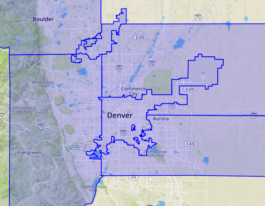
Figure 12.6 Selected Counties around Denver County

12.3.3.2. Major Roads

Much like adjacent county polygons, having major roads to display can be helpful for visualizations. Listing 12.26 uses a CTE (c) to first aggregate the six (6) polygons (ST_Union(geom)) before performing the containment search. A PRIMARY KEY and spatial index is added for good measure.

Listing 12.26 Create osm_denver.major_roads for Denver and surrounding area

CREATE TABLE osm_denver.major_roads AS
WITH c AS (
SELECT ST_Union(geom) AS geom
    FROM osm_denver.county
)
SELECT r.*
    FROM c
    INNER JOIN osm.road_line r
        ON ST_Contains(c.geom, r.geom)
          AND r.major
;

ALTER TABLE osm_denver.major_roads
    ADD CONSTRAINT pk_osm_denver_major_roads
    PRIMARY KEY (osm_id)
;

CREATE INDEX gix_osm_denver_major_roads
    ON osm_denver.major_roads USING GIST (geom)
;

The county polygon and major road data provides a simple visualization of the area shown in Figure 12.7.

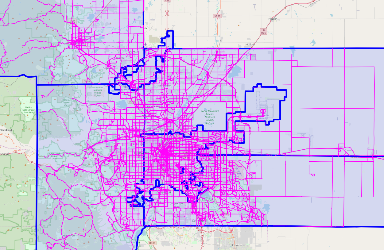
Figure 12.7 Thematic Roads and selected counties around Denver County.

12.3.4. Cleanup

The code in the previous sections created some tables that are no longer needed. These artifacts are dropped in Listing 12.27.

Listing 12.27 Drop unnecessary objects from osm_denver schema

DROP TABLE osm_denver.focus;
DROP TABLE osm_denver.road_line_bbox;
DROP TABLE osm_denver.road_line_contain;

The query in Listing 12.28 shows the tables created in the osm_denver table take up only 51 MB.

Listing 12.28 Query to show the size on disk of the data in the osm_denver schema

SELECT s_name, table_count, size_pretty
    FROM dd.schemas
    WHERE s_name = 'osm_denver'
;

┌────────────┬─────────────┬─────────────┐
│   s_name   │ table_count │ size_pretty │
╞════════════╪═════════════╪═════════════╡
│ osm_denver │           6 │ 51 MB       │
└────────────┴─────────────┴─────────────┘

The query in Listing 12.29 shows the six (6) tables created in the osm_denver schema.

Listing 12.29 Query to examine row count and size on disk of tables in osm_denver schema

SELECT s_name, t_name, size_pretty, rows, bytes_per_row
    FROM dd.tables
    WHERE s_name = 'osm_denver'
    ORDER BY t_name
;

┌────────────┬──────────────────┬─────────────┬────────┬────────────────────┐
│   s_name   │      t_name      │ size_pretty │  rows  │   bytes_per_row    │
╞════════════╪══════════════════╪═════════════╪════════╪════════════════════╡
│ osm_denver │ building_polygon │ 46 MB       │ 186062 │  261.2201094258903 │
│ osm_denver │ county           │ 200 kB      │      6 │ 34133.333333333336 │
│ osm_denver │ major_roads      │ 9352 kB     │  41107 │ 232.96392341936897 │
│ osm_denver │ natural_point    │ 12 MB       │ 164843 │  76.82966216339183 │
│ osm_denver │ road_line        │ 14 MB       │  74269 │  204.0582207919859 │
│ osm_denver │ water_line       │ 520 kB      │   1482 │ 359.29824561403507 │
└────────────┴──────────────────┴─────────────┴────────┴────────────────────┘

Warning

The table osm_denver.major_roads does not follow the preferred naming convention. Listing 12.30 fixes this by renaming the table to osm_denver.road_major_line.

Listing 12.30 Rename major_roads table

ALTER TABLE osm_denver.major_roads
   RENAME TO osm_denver.road_major_line;

12.3.5. Dump

To query in Listing 12.31 uses pg_dump to create a compressed extract with the data. This process was explained in Section 12.2.4.

Listing 12.31 Use pg_dump to save and share the osm_denver schema

pg_dump --no-owner --no-privileges -Z6 \
    -n osm_denver -n pgosm \
    -d pgosm \
    -f osm_denver.sql.gz

Returning to our project assumptions, the prepared data now includes the surrounding Denver Metro areas for seamless visualization. The cleanup and dump phases promoted a tidy database that can be queried easily and quickly, as well as enables easy sharing of the data with others.